Article Text

Abstract
Objective Compare performance between an injury prediction model categorising predictors and one that did not and compare a selection of predictors based on univariate significance versus assessing non-linear relationships.
Methods Validation and replication of a previously developed injury prediction model in a cohort of 1466 service members followed for 1 year after physical performance, medical history and sociodemographic variables were collected. The original model dichotomised 11 predictors. The second model (M2) kept predictors continuous but assumed linearity and the third model (M3) conducted non-linear transformations. The fourth model (M4) chose predictors the proper way (clinical reasoning and supporting evidence). Model performance was assessed with R2, calibration in the large, calibration slope and discrimination. Decision curve analyses were performed with risk thresholds from 0.25 to 0.50.
Results 478 personnel sustained an injury. The original model demonstrated poorer R2 (original:0.07; M2:0.63; M3:0.64; M4:0.08), calibration in the large (original:−0.11 (95% CI −0.22 to 0.00); M2: −0.02 (95% CI −0.17 to 0.13); M3:0.03 (95% CI −0.13 to 0.19); M4: −0.13 (95% CI −0.25 to –0.01)), calibration slope (original:0.84 (95% CI 0.61 to 1.07); M2:0.97 (95% CI 0.86 to 1.08); M3:0.90 (95% CI 0.75 to 1.05); M4: 081 (95% CI 0.59 to 1.03) and discrimination (original:0.63 (95% CI 0.60 to 0.66); M2:0.90 (95% CI 0.88 to 0.92); M3:0.90 (95% CI 0.88 to 0.92); M4: 0.63 (95% CI 0.60 to 0.66)). At 0.25 injury risk, M2 and M3 demonstrated a 0.43 net benefit improvement. At 0.50 injury risk, M2 and M3 demonstrated a 0.33 net benefit improvement compared with the original model.
Conclusion Model performance was substantially worse in the models with dichotomised variables. This highlights the need to follow established recommendations when developing prediction models.
- Injury
- Prevention
- Risk factor
- Neuromuscular
Data availability statement
Data are available on request and procurement of applicable, data sharing agreements from the US Defense Health Agency (applications for MDR DSAs can be found at health.mil).
This is an open access article distributed in accordance with the Creative Commons Attribution Non Commercial (CC BY-NC 4.0) license, which permits others to distribute, remix, adapt, build upon this work non-commercially, and license their derivative works on different terms, provided the original work is properly cited, appropriate credit is given, any changes made indicated, and the use is non-commercial. See: http://creativecommons.org/licenses/by-nc/4.0/.
Statistics from Altmetric.com
WHAT IS ALREADY KNOWN ON THIS TOPIC
Dichotomising predictors often result in suboptimal prediction models (poor model fit, calibration in the large, calibration slope and discrimination) compared with models that keep predictors continuous.
Dichotomising predictors reduces the ability to accurately identify tactical athletes at risk for injury.
WHAT THIS STUDY ADDS
This study provides real-world examples of how model performance is affected with these suboptimal practices and how much better injury prediction science can be when using proper methods.
HOW THIS STUDY MIGHT AFFECT RESEARCH, PRACTICE OR POLICY
It is imperative to keep injury predictors continuous when evaluating injury risk, which is currently not standard practice.
Personalising prediction models that are informative and simple to implement are still possible when using continuous-level predictors.
Introduction
Injury to the musculoskeletal system enacts a significant health burden at both the individual and societal levels.1 This has prompted an entire line of research aimed at identifying methods to accurately predict which individuals are at higher risk for injury.2 3 Valid prediction models have the potential to identify targets for intervention and prevention strategies aimed at reducing injuries. A substantial problem currently in the field of modelling prediction (ie, risk) within medicine in general revolves around the use of suboptimal practices in the planning, development and execution of these studies4, and the sports and musculoskeletal injury literature are no exception.5 This poor practice can lead to substantial bias. This problem has also led to the development of guidelines and checklists to improve the quality of executing prediction modelling studies.6–8
Two practices that go against published recommendations, but continue to be common, are dichotomising continuous-level predictors 9–11 and choosing predictors based on their significance in univariable analysis.12 The arguments for these practices are that they simplify the process, create clearly defined decision points and are easier to implement in real-world settings. For example, our prior research found ankle dorsiflexion asymmetry >5° to be a predictor of injury risk in a multivariate model.13 14 Although this provides a simple and easy method to interpret cut-off value, these practices oversimplify the process, potentially including or excluding relevant predictors, and needlessly decreasing the predictive value of the individual variable.2 15 These practices may also limit the validity of injury prediction models, considering the multivariate nature of the musculoskeletal injury and the complexity and interrelationship of predictors associated with injury risk.2 15
The historical use of dichotomising continuous predictors16 or using univariate analysis to prioritise predictors of interest4 12 may be an oversimplification that could come with consequences to model performance.17 In fact, while the findings may seem easier to implement, they could also be incorrect, failing to fully account for the complexity of injuries.2 18 Our objective was to investigate how both dichotomisation of continuous predictors and selection of predictors based on univariable significance influence model development and subsequent performance. Using a prediction model previously developed using univariable screening and dichotomisation of continuous predictors, we aimed to quantify the impact on predictor selection and performance of the prediction model performance if best practice modelling approaches were implemented.19 Specifically we sought to (1) determine if and how model performance would improve if continuous predictors were not dichotomised, (2) determine how model performance would change if predictors were selected appropriately rather than based only on univariable significance and (3) demonstrate that a personalised and pragmatic prediction model can still be generated when continuous predictors were not dichotomised.
Methods
Study design and overview
This is a validation and replication study. Our team originally derived a model for predicting musculoskeletal injury by dichotomising continuous predictors and choosing predictors based on univariable significance.13 Briefly, the original study enrolled 1466 military service members who, at study entry, were considered healthy and without any physical duty restrictions. Following initial recruitment, 11 withdrew from the study, and 25 had an undisclosed injury at baseline, leaving 1430 final participants. At baseline, 158 potential predictors of injury risk were collected from participants. Injury surveillance took place over 1 year within two diverse subgroups based on occupational requirements. The first cohort consisted of 320 US Army Rangers14 and the second cohort consisted of 1146 regular US Army Soldiers.13
Predictors
Possible predictors included physical performance measures (Functional Movement Screen [FMS], Y-Balance Test for the upper and lower quarter, and hop testing),20–22 medical history to include prior injuries, surgeries and lost work days due to a previous injury, and perceived recovery using the Single Assessment Numerical Evaluation (SANE; 0%–100%). Physical fitness scores that included sit-ups, push-ups and a two-mile run were also collected based on most recent test score at the beginning of the data collection period (within 6 months).23 24 Specific details for the physical performance testing have been published.25
Outcome definition
An injury was defined in the original study as a care-seeking encounter in which an injury diagnosis code (International Classification of Diseases, Ninth Edition) was rendered in the participant’s electronic medical record with associated time lost from military duties.26 Time loss was captured from the e-profile database within the Military Operational Data System (MODS), which lists the total number of days assigned to restricted duty and reason for that restriction.
Statistical analyses
Participant characteristics were described using median (min, max) for continuous predictors, and frequencies and percentages for categorical predictors. Injury incidence was calculated per 1000 military exposure days.
Summary of statistical approach in original prediction model
The original model was developed using logistic regression to calculate individual risk of injur. All continuous predictors were dichotomised at cut points based on values from literature or thresholds determined during the data analyses (eg, median cut point, receiver operating characteristic curves). Please refer to the model development section for further information on each predictor cut point (ie, threshold). All count and nominal predictors were collapsed into binary predictors. Predictors were originally chosen based on significance in univariable testing (t-test with p<0.20 or OR>2.0) and then entered into a final multivariable model where only predictors with a p≤0.05 were retained. Participants who sustained an injury, but did not seek medical care, were excluded from the model. A simplified tool was then created based on a count of the presence of the resulting 11 predictors that were retained in the model (ranging from 0 to 11), with a score of 7 or more used as an indication that an individual is at high risk for injury.
Statistical approach for model validation (new approach)
All data were investigated for missingness prior to analyses, with missing data being low (age: 0%, military years: 0%, body mass index: 0%, SANE: 0%, Y-Balance Test (Lower and Upper Quarter: <0.1%), 2 Mile Run 2%, Sit Ups: 2%). Complete-case analyses were performed.
Prior to model development, continuous predictors were assessed for non-linear relationships with sustaining a musculoskeletal injury through restricted cubic splines using three, four and five knots.27 A restricted cubic spline is a non-linear piecewise polynomial (non-linear calculation) joined at specific knots throughout the data. Knots are quantile mark points in which each segment (between each knot) is assessed for potential non-linear relationships.27 The range of data is joined at each successive knot, allowing for different non-linear relationships to be assessed throughout the entirety of the data.27 A data-driven approach using Akaike information criterion was used to determine potential non-linear transformations. It was determined that military service years, number of injuries over the prior year and timed sit-ups were best explained by a non-linear relationship of 3 knots, while two-mile run time was best explained by four knots (online supplemental appendix SA.1.1). All other continuous predictors had a linear relationship with sustaining a musculoskeletal injury.
Supplemental material
Sample size calculation
A priori sample size calculations were performed prior to model development, using the R package pmsampsize. Sample size requirements for developing a multivariable risk prediction model involve specifying three components: the anticipated model R2, the injury prevalence, and the total number of predictor parameters.28 As we used an existing dataset, with a fixed sample size of 1430 participants, the number of predictors was determined through the sample size calculations. The Cox-Snell R2 of 0.12 from the originally developed model was used,13 and the prevalence of musculoskeletal injury was 0.34. It was determined that a total of 21 predictor parameters could be examined for potential inclusion in the prediction model.
Model development
The Transparent Reporting of a multivariable prediction model for Individual Prognosis or Diagnosis (TRIPOD) was followed for reporting all aspects of model development.19 All models were fit using logistic regression, with the occurrence of a time loss musculoskeletal injury as the outcome, and internally validated with 2000 bootstraps to correct for performance optimism. The original model (M1) choose variables based on univariable significance and dichotomised all 11 predictor variables. The first variation of the model (M2) kept the predictor continuous (instead of dichotomising) but assumed all predictors were linear. The next model (M3) kept predictors continuous and appropriate non-linear transformations were accounted for (rather than assuming all relationships with linear predictors would be linear). Model 4 was developed to further highlight the impact of dichotomising predictors even when predictors were selected the recommended proper way (based on evidence to support the variable and clinical reasoning/consensus) rather than based on univariable significance. This model resulted in 4 additional predictor variables (15 total) being added to the model (none of the original ones excluded), but kept them dichotomous like the original model. Finally, one last model (M5) was created following best practices in all regards; predictors were chosen based on rationale from the literature and clinical expertise (like M4) and all predictors were kept continuous along with accounting for non-linear transformations (like M3).
The five models included:
Model 1: The original model13 included the following 11 predictors chosen based on univariable significance (p>0.25): (1) age (≥ 26.0), (2) sex, (3) prior injury (≥1), (4) SANE (≤92.5%), (5) Profile Time During Past Year (>1), (6) Pain on Movement Tests (>= 1), (7) Dorsiflexion Asymmetry (≥4.5°), (8) YBT-LQ Anterior Reach Distance (≤72.0%), (9) YBT-UQ Superolateral Reach Distance (≤80.1%), (10) YBT-UQ Inferolateral Asymmetry (≥7.75%), (11) 2 Mile Run Time (≥919.5 s).
Model 2: The original model except for all continuous predictors were kept continuous and was assumed to be linear.
Model 3: The original model except for all continuous predictors were kept continuous and non-linear transformation was conducted when appropriate.
Model 4: A model developed conforming to the a priori sample size calculations. Based on rationale from the literature and clinical reasoning, 15 predictors (continuous variables; 11 from the original model plus 4 new ones) were dichotomised based on the original study cut points. The additional four prredictors included: (1) body mass index (≥ 27.5), (2) Number of Sit Ups (≤85.5), (3) Triple hop test score (<= 450), (4) FMS total score (≤14).
Model 5: Predictor variables from M4 and treatment of continuous variables as was done in M3 (keeping continuous predictors as continuous; proper non-linear transformation when appropriate).
Following model development and internal validation, a dynamic multivariate nomogram was created with the rms package.29 Because coefficients alone are less helpful in real-world practice, nomograms facilitate implementation of findings by reducing statistical prediction models to a single numeric estimate of the probability of the event. As values for predictors are adjusted in the nomogram, the user can see this estimate for the probability of the event change accordingly. A probability of 0 indicates that injury is unlikely whereas a score closer to 1 indicates a strong likelihood of injury.
Model performance
Model performance was investigated by assessing Nagelkerke R2, Brier score, calibration in the large, calibration slope and discrimination. The Brier score is a prediction performance measure that combines discrimination and calibration. A lower score is improved performance. Calibration in the large assesses the average predicted outcome compared with the average actual outcome, with a calibration in the large of zero demonstrating optimal performance. Calibration slope measures agreement between predicted risks from the model and what was observed, while discrimination evaluates how well the model differentiates between those with and without the outcome. Calibration was plotted graphically with the the predicted risk against the observed outcome using a loess smoother. Calibration shows the predicted risk graphically against the observed outcome, displaying the calibration intercept and calibration slope. Discrimination was evaluated by the area under receiver operating characteristic curve (AUC). An AUC of 0.5 implies the model is no better than random guessing. An AUC of 1.0 demonstrates perfect (100%) discrimination.
Decision curve analysis, by using 10-fold cross-validation, was performed to determine the net benefit of incorporating the arm injury prediction model into clinical practice.30 31 The net benefit is the fraction of true positives gained by making decisions based on predictions over a range of plausible risk thresholds.30 31 The a priori risk threshold probability was defined in cooperation with stakeholder groups and from review of previous military injury risk literature.14 32 33 As injury risk can vary between military personnel, the net benefit was calculated through a range of predicted risks, ranging from 0.25 to 0.50.14 32 33 For each model, net benefit was compared with strategies that assume all military personnel are at high risk (‘treat all’) and assuming all are at low risk (‘treat none’).31 34 To put in further clinical context, ‘treat all’ would be equivalent to providing every soldier with an individualised injury prevention programme targeting these risk factors. On the other hand, ‘treat none’ would entail ‘watchful waiting’ or potentially providing only generic programmes to all military personnel. These analyses are performed to help improve resource allocation (ie, providing unnecessary individualised injury prevention programmes) precision of efforts towards at-risk military personnel.31 34 All analyses were performed in R V.3.5.1. The rms and Hmisc packages were used for prediction model development, the caret package was used for internal validation, the CalibrationCurves package was used to visualise calibration, and the rmda package was used for decision curve analyses and plotting.
Multivariable nomograms
Multivariable nomograms were created for the original model replicated with continuous predictors and non-linear transformations (M3) and also for the model using all optimal practices (M5) found in SA1.7 to SA1.8. A dynamic multivariable nomogram for the newly developed model was created using the rms package 29 (link and legend provided in SA1.9).
Patient and public involvement statement
This was a secondary analysis of prior collected data. As such, no patients or other public stakeholders were involved in this study.
Results
A total of 1466 military personnel were included in this cohort. After removing 11 that withdrew and 25 with an undisclosed injury at baseline, 1430 remained for the final analysis (table 1). Injury incidence was 1.3 per 1000 military exposure days with 478 personnel sustaining an injury during the study period.
Participant descriptive statistics
Comparison of model performance
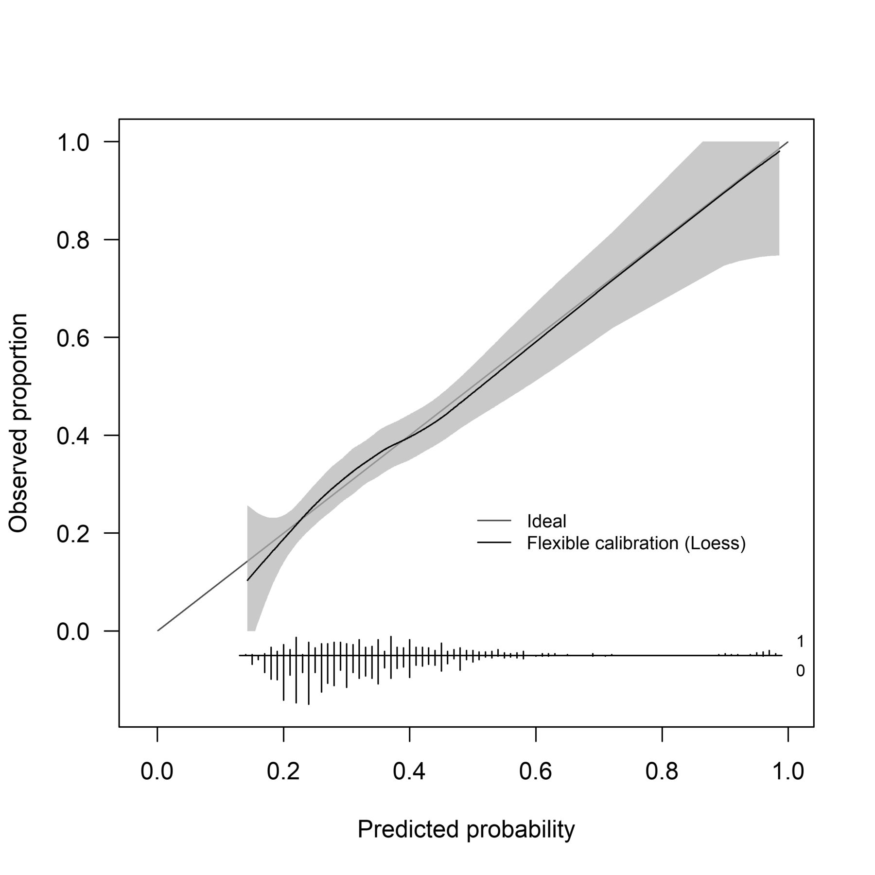
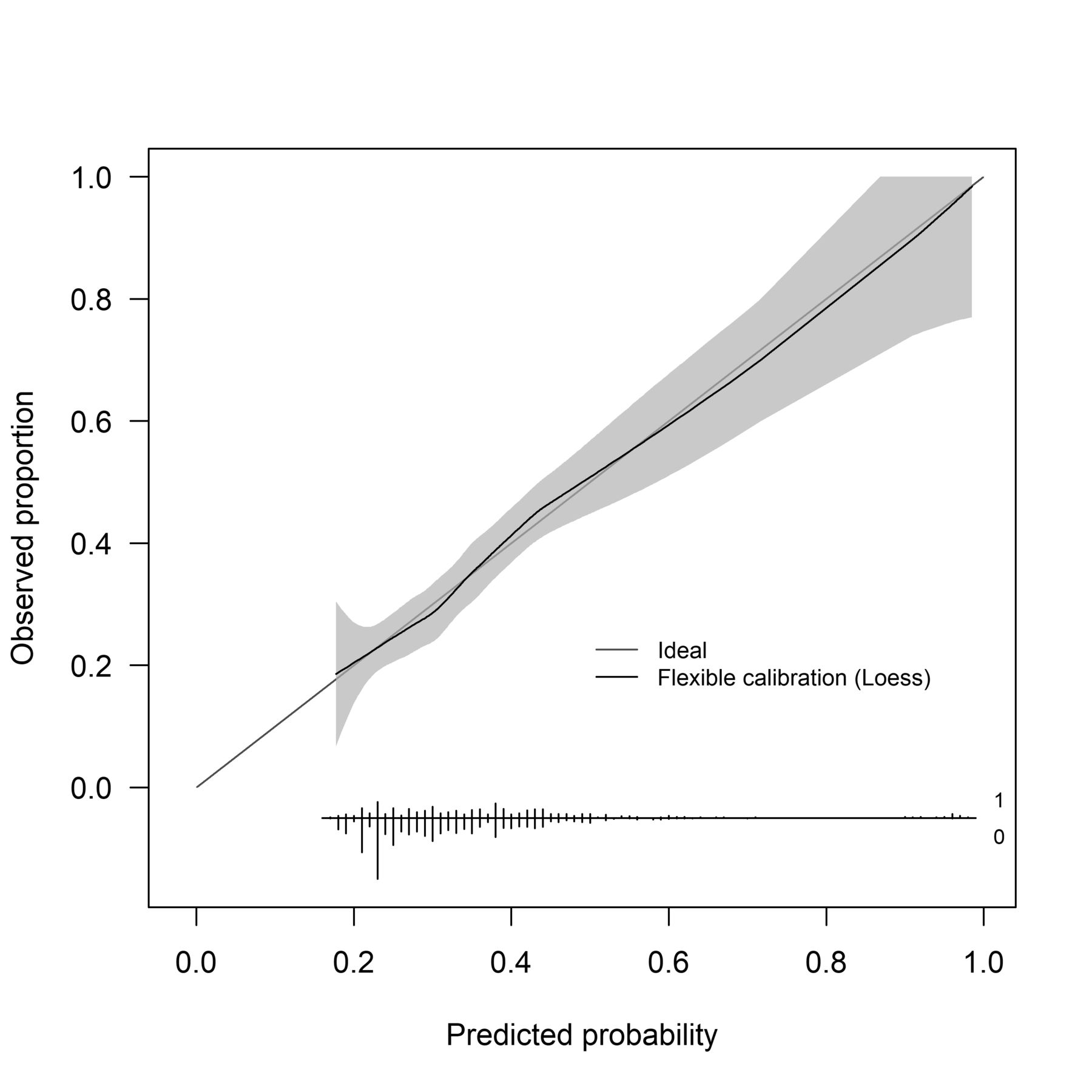
The original model replicated with continuous predictors with linearity assumed (M2) and non-linear transformations (M4) demonstrated improved overall model performance compared with the original model, with a 0.26–0.27 improvement in AUC, a 0.06–0.13 improvement in calibration slope, 0.49–0.57 increase in R2, and a 0.08–0.09 improvement in Brier score.13 Including a greater number of predictors, but keeping them dichotomised (M3) demonstrated similar performance to the original model (table 2). The original model (M1) did not calibrate below 0.20 risk (figure 1). The M2 model did not demonstrate stable calibration across risk thresholds (figure 2). The M4 model did not calibrate below 0.20 risk (figure 3). Wide CIs were noted for M3 below 0.30 risk (figure 4). Finally, the optimal model (M5) performed similarly to M3 (figure 5). Full mathematical descriptions of all models are in the online supplemental appendix (SA1.2-SA1.6).
Comparing model performance of the injury prediction models

Calibration slope of original developed model (M1). Calibration is the relationship between predicted and actual probability of the event. The calibration slope plots the predicted risk graphically against the observed outcome; displaying the calibration intercept and calibration slope. perfect calibration would result in a 45° line. Within this calibration plot, risk does not begin until 0.20. What this clinically means is that everyone’s risk cannot be lower than 0.20. Individuals with little risk of injury may be inappropriately referred for clinical care.

Calibration slope of original developed model replicated with continuous predictors; linearity assumed (M2). Calibration is the relationship between predicted and actual probability of the event. The calibration slope plots the predicted risk graphically against the observed outcome; displaying the calibration intercept and calibration slope. perfect calibration would result in a 45° line. The predicted risk is lower between 0.20 and 0.40, compared with the actual risk for these individuals. What this means clinically is that these individuals would be under estimated for their true risk of injury, and potentially not referred to the appropriate clinical care or injury prevention strategies.

Calibration slope of original developed model replicated with continuous predictors and non-linear transformations (M3). Calibration is the relationship between predicted and actual probability of the event. The calibration slope plots the predicted risk graphically against the observed outcome; displaying the calibration intercept and calibration slope. Perfect calibration would result in a 45° line. Predicted risk between 0.20 and 0.40 is slightly lower than actual risk, which may alter clinical decisions for individuals within this risk threshold.
Calibration slope when using best practices to choose predictors (added several new predictors), but keeping them all dichotomised (M4). Calibration is the relationship between predicted and actual probability of the event. The calibration slope plots the predicted risk graphically against the observed outcome; displaying the calibration intercept and calibration slope. Perfect calibration would result in a 45° line. Within this calibration plot, risk does not begin until 0.20. What this clinically means is that everyone’s risk cannot be lower than 0.20. Individuals with little risk of injury may be inappropriately referred for clinical care.

Calibration slope of optimal model developed based on appropriately chosen predictors, keeping predictors continuous and conducting appropriate non-linear transformations (M5). Calibration is the relationship between predicted and actual probability of the event. Perfect calibration would result in a 45° line. The calibration slope plots the predicted risk graphically against the observed outcome; displaying the calibration intercept and calibration slope. This calibration model demonstrates risk from 0.00 to 1.0, and has the most uniform predicted risk to the actual risk. Predicted risk between 0.20 and 0.40 is lower than actual risk, which may alter clinical decisions for individuals with the least risk of injury.
Decision curve analyses
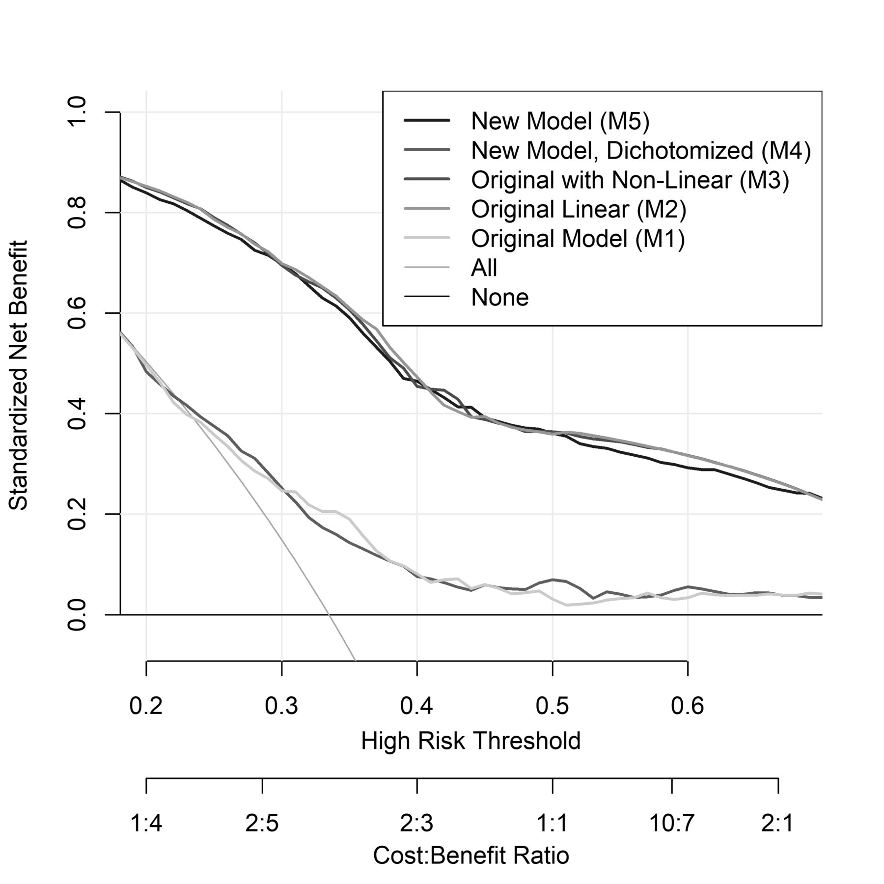
The original model with continuous predictors and linearity assumed (M2) and the original model with non-linear transformations (M3) demonstrated a greater net benefit at the a priori range of 0.25 to 0.50 injury risk compared with the original model (M1) and larger dichotomised model (M4) (table 3 and figure 6). At 0.25 injury risk, the M3 model demonstrated a 0.47 net benefit improvement compared with the original model (M1). In other words, out of 100 military personnel the original model with continuous predictors and non-linear transformations and the newly developed model would improve injury identification by 47 military personnel compared with the original model. At 0.50 injury risk, the M3 demonstrated a 0.36 net benefit improvement compared with the original model (M1). In other words, out of 100 military personnel the M3 would improve injury identification by 36 military personnel compared with the original model.
Net benefit of military personnel injury risk identification using a ‘treat all’ approach, the original model, the original model with continuous predictors and non-linear transformations, and a newly developed model

Decision curve for the prediction models to predict injury risk in military personnel. The figure reports the expected net benefit compared with not predicting injuries. ‘Treat all’ assumes that all military personnel are at a high risk for injury and should be intervened on, while treat none assumes that all military personnel are at a low risk for injury and NO interventions should be performed. The threshold probability was defined as the population risk of injury within military personnel of 0.25–0.50. The models keeping predictors continuous (M2, M3, M5) non-linear transformations (M3, M5) all demonstrated improved net benefit (ie, correct injury identification) compared with ‘treat all’ and the original (M1) model and the original model with further added dichotomised predictors (M4) at these threshold probabilities.
Discussion
The main findings of this study were that the original model (M1) with dichotomised predictors demonstrated decreased performance compared with models that maintained continuous models as continuous (M2 and M3). Even when choosing predictors, the proper way (rather than relying on univariable significance) model performance was still suboptimal when those predictors remained dichotomised (M4). Model performance did not improve with new predictors compared with the original model, suggesting that properly using continuous predictor variables (eg, not dichotomising and not assuming linearity) may be a more important task than predictor selection when developing optimal injury prediction models in this population.
Our results highlight stark differences in model derivation and performance when using different approaches. When replicating the original model (M1) with proper use of predictors (eg, not dichotomising continuous predictors (M2) and assessing for non-linear relationships (M3)), all model prediction performance metrics (ie, discrimination, calibration and model fit) and clinical decisions improved. These findings support previous literature detailing how artificially dichotomising continuous predictors lose information, decrease prediction precision and impair clinical decisions.9–11 16 When appropriately choosing predictors based on clinical reasoning and supporting evidence but still dichotomising the continuous predictors (M4), model performance was still suboptimal and similar to the original model. When those same continuous predictors were accounted for appropriately in the model (M5), the performance improved substantially and was similar to M3. This suggests that the predictors originally chosen were appropriate and robust for predicting injuries, even if the way they were initially selected was based on univariable relationships with injury. Conceptually, using dichotomised predictors, even when predictors were selected appropriately, was almost no better than taking a ‘treat all’ approach without an attempt to identify more personalised injury risk. The constructs for predicting injury were correct, but their original definition and use in the model were suboptimal. These results highlight in a practical way how the many advances in prediction modelling approaches made over recent years can apply to the sports sciences. Statistical guidelines provide warning about the potential consequences of various substandard approaches to deriving prediction models.9–11 Our results highlight real-world examples of these consequences.
One common argument for dichotomising predictors is that they are simpler to interpret. But continuous predictors are continuous for a reason, often reflecting a wide range of values. For example, a cut point of 93 for perceived recovery after injury (0 indicating no recovery to 100 indicating full recovery) places individuals with a score of 92.5 and 10 in the same category, below the dichotomous cut-point. The model cannot discriminate between the wide range of values once it has been dichotomised, leading to an improper and biased assessment of the utility of that variable as a predictor. In the original injury prediction model, the 11 final predictors were entered into a prognostic accuracy profile to calculate sensitivity, specificity and likelihood ratios. The appeal was in the value for the stakeholder (eg, the individual, the unit commander), who could simply assess the change in injury likelihood by counting the number of predictors present.
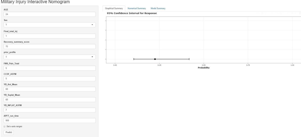
There are solutions however for personalising prediction models and making them easier to interpret. Multivariable nomograms can plot all predictors, including continuous predictors and provide similar probabilities. This can improve the precision of the prediction models at the single-person level and improve interpretation of interdependent relationships of the predictors. For example, as values from continuous predictors go up and down, the end-user can see how the probability of injury changes. Online supplemental appendix (SA1.13–15) provide a multivariable nomogram tool created specifically for the two additional developed models. An example of the dynamic nomogram is provided in figure 7 We feel this is a more meaningful and accurate tool to inform individual risk for injury. Another framework to help simplify this could be to develop certain actions based on specific risk thresholds. Using a traffic light example which is common in military settings, a risk score of <0.25 may be interpreted as a ‘green light’ (low risk, no action needed), a score of 0.25–0.50 as a ‘yellow light’ (moderate risk) and a score of >0.50 as ‘red light’ (high risk). Yellow light individuals could be flagged for further assessment and treatment. Red light individuals could be held back from returning to duty until identified risk factors were properly addressed and a lower risk score was observed.

Example of the multivariate injury dynamic nomogram. Probability of injury is approximately 22.5% (95% CI of 10.6% to 41.8%) when a 24-year-old male has one previous injury in the military, a recovery score of 70, was on profile the previous year, five movements reported pain, a 5° asymmetry in ankle dorsiflexion, 68% limb length on the Y-Balance anterior reach, 68% limb length on the Y-Balance upper quarter superolateral reach, and 7% limb length asymmetry on the Y-Balance upper quarter inferolateral reach and completes the 2 mile run in a time in 868 s (14 min, 29 s). (More examples in online supplemental appendix).
It should be noted that these models used a complete case analysis, as the prevalence of missing data was low, with a missing mechanism of missing at random. However, data prototypically have a higher missing prevalence, and require methods to handle missing data bias.35 In these cases, multiple imputation is advised.36 Multiple imputation involves predicting (ie, imputing) missing values to estimate the distribution of the data.36 37 Imputation is performed multiple times to account for uncertainty in the missing data, creating many individual data sets. Data sets are analysed independently, with each dataset aggregated into one uniform result.35 37
This study has limitations. First, the original cohort was broken down into two occupational subgroups,13 14 each with its own independent prediction model. The replication of the previous model and the derivation of the new model occurred using the entire cohort. Performing an internal–external validation strategy would have improved generalisability for the analyses38; however, this was not possible with the relatively small size of the Army Ranger unit. Including everyone in the cohort makes the results more practical, as all these individuals would be present in real-world use of the model. However, future external validation is required to understand the generalisability of these models to other military populations.
Conclusion
Our previously derived injury prediction model based on dichotomous cut points for most predictors was no better than not trying to predict individualised injury risk (eg, treat all). It demonstrated worse performance compared with proper statistical approaches to modelling injury risk that properly accounted for continuous-level predictors. When the original predictors were kept continuous, the model performed extremely well. Although models using continuous predictors may be harder to interpret, the use of multivariable nomograms and categorical frameworks of injury risk can provide an equally meaningful individualised risk profile. This highlights even further the need to follow best practices and guidelines for developing prediction models and to clearly report the methods to maximise transparency and reproducibility.
Data availability statement
Data are available on request and procurement of applicable, data sharing agreements from the US Defense Health Agency (applications for MDR DSAs can be found at health.mil).
Ethics statements
Patient consent for publication
Ethics approval
This study involves human participants and was approved by US Army’s Regional Health Command Pacific Institutional Review BoardApproval # 211011. Participants gave informed consent to participate in the study before taking part.
References
Supplementary materials
Supplementary Data
This web only file has been produced by the BMJ Publishing Group from an electronic file supplied by the author(s) and has not been edited for content.
Footnotes
Twitter @danrhon
Contributors DIR, GSB and GSC contributed to the idea and statistical approach; DIR and DST procured funding and the data. All authors contributed to the interpretation of the findings, writing and editing of the initial draft, and final approval of the final manuscript. DIR acts as guarantor of this work.
Funding This research was supported by the Defense Medical Research and Development Program and Military Operational Medicine Research Programs (D10_I_AR_J5_951) and also in part by the Uniformed Services University, Department of Physical Medicine and Rehabilitation, Musculoskeletal Injury Rehabilitation Research for Operational Readiness (MIRROR HU00011920011).
Disclaimer The view(s) expressed herein are those of the author(s) and do not necessarily reflect the official policy or position of Brooke Army Medical Center, the US Army Office of the Surgeon General, the Department of the Army, the Defense Health Agency, the Department of Defense, the Uniformed Services University of the Health Sciences, nor the US Government.
Competing interests None declared.
Patient and public involvement Patients and/or the public were not involved in the design, or conduct, or reporting, or dissemination plans of this research.
Provenance and peer review Not commissioned; externally peer reviewed.
Supplemental material This content has been supplied by the author(s). It has not been vetted by BMJ Publishing Group Limited (BMJ) and may not have been peer-reviewed. Any opinions or recommendations discussed are solely those of the author(s) and are not endorsed by BMJ. BMJ disclaims all liability and responsibility arising from any reliance placed on the content. Where the content includes any translated material, BMJ does not warrant the accuracy and reliability of the translations (including but not limited to local regulations, clinical guidelines, terminology, drug names and drug dosages), and is not responsible for any error and/or omissions arising from translation and adaptation or otherwise.