Article Text

Abstract
Objectives Determine how to assess the cumulative effect of training load on the risk of injury or health problems in team sports.
Methods First, we performed a simulation based on a Norwegian Premier League male football dataset (n players=36). Training load was sampled from daily session rating of perceived exertion (sRPE). Different scenarios of the effect of sRPE on injury risk and the effect of relative sRPE on injury risk were simulated. These scenarios assumed that the probability of injury was the result of training load exposures over the previous 4 weeks. We compared seven different methods of modelling training load in their ability to model the simulated relationship. We then used the most accurate method, the distributed lag non-linear model (DLNM), to analyse data from Norwegian youth elite handball players (no. of players=205, no. of health problems=471) to illustrate how assessing the cumulative effect of training load can be done in practice.
Results DLNM was the only method that accurately modelled the simulated relationships between training load and injury risk. In the handball example, DLNM could show the cumulative effect of training load and how much training load affected health problem risk depending on the distance in time since the training load exposure.
Conclusion DLNM can be used to assess the cumulative effect of training load on injury risk.
- training load
- injury
- simulation
- time-to-event analysis
Data availability statement
Data are available in a public, open access repository. Data are available upon reasonable request. All data relevant to the study are included in the article or uploaded as supplementary information. All data relevant to the study are included in the article, are available as supplementary files, or available upon reasonable request. The anonymous training load variable from the Norwegian Premier League football data, and all statistical programming code, is available in a GitHub repository. The anonymised Norwegian elite youth handball data are available upon reasonable request.
This is an open access article distributed in accordance with the Creative Commons Attribution Non Commercial (CC BY-NC 4.0) license, which permits others to distribute, remix, adapt, build upon this work non-commercially, and license their derivative works on different terms, provided the original work is properly cited, appropriate credit is given, any changes made indicated, and the use is non-commercial. See: http://creativecommons.org/licenses/by-nc/4.0/.
Statistics from Altmetric.com
WHAT IS ALREADY KNOWN ON THIS TOPIC
Training load seems to affect the risk of injury in team sports.
Time since exposure to training load may determine the strength and the direction of training load’s effect on injury risk.
The ability of current methodology to assess above-mentioned effects is limited.
WHAT THIS STUDY ADDS
Distributed lag non-linear models (DLNMs) were superior to all methods compared and could determine the cumulative effect of past training load.
The exponentially weighted moving average (EWMA) performed better than the rolling average and robust exponential decreasing index.
The difference between the acute:chronic workload ratio and week-to-week percentage change was negligible.
HOW THIS STUDY MIGHT AFFECT RESEARCH, PRACTICE AND/OR POLICY
Researchers can estimate the effects of training load on the risk of injury in team sports using DLNM.
More consistent methodology in training load and injury risk studies will improve comparability and reproducibility.
Introduction
In recent years, researchers have attempted to determine the effect of training load on the risk of sports injuries and other sports-related health problems.1 Training load is the physical exertion that the athlete has been exposed to and is a combination of the exposure itself (external load) and the physiological and psychological stressors applied to the athlete in response to the exposure (internal load).2 Relationships between risk factors and sports injuries are often complex,3 as the effect of risk factors may depend on the presence or absence of other risk factors,3 the current state of the athlete,4 and they may also act non-linearly on the risk of injury.4
Assessing training load poses additional challenges.5 6 It is a multidimensional construct that can be measured in multiple ways.7 Hypotheses suggest that not only the amount of training load, but also the relative change in training load affect injury risk.5 Balanced training load exposure may both cause and protect against injury through building fitness and fatigue.8 A central concern is that training load is a time-varying exposure with special properties.5 9 The training load exposure on the current day affects injury risk directly—an athlete cannot sustain a sports injury without participating in a sporting activity.5 Training load may, however, also be a so-called time-lagged effect.10 The training load on the previous day may contribute to the injury risk on the current day. To further add complexity, training load is likely to have a protracted time-lagged effect.11 The injury risk at any given time is the result of multiple training load exposure events of different intensities sustained in the past.12 In summary, no single training load exposure event is thought to affect injury risk in isolation, rather it is the long-term exposure to training load leading up to the event collectively that is assumed to influence injury occurrence.
To meet these assumptions, previous research has addressed some of the complexities of modelling training load statistically.9 13 A statistical model is a generalisation that is unlikely to tailor the prognostic course of an individual accurately,14 but it may inform researchers and clinicians about causation and patterns of injury risk. Among others, statistical solutions have been proposed to handle the time-varying effects,9 the potential for non-linear effects,15 the cumulative effect,13 16 and the effect of relative training load17 in the risk of injury. While statistical models and approaches have been recommended to handle these challenges in isolation, it is still unknown how to explore all the raised challenges in symphony. That is, accounting for time-varying effects, non-linear effects and cumulative effects simultaneously.
We aimed to determine how to model training load when assessing its cumulative effect on the risk of injury or health problems in a longitudinal team sports study.
Materials and methods
First, we ran a simulation study based on football data with internal training load measures to compare the performance of different statistical approaches. Then, we implemented the best performing approach on a handball dataset with training load and injury measures to demonstrate how it can be used in practice.
Football data simulation
To compare the performance of different statistical approaches, it is common to run stochastic simulations.18 We constructed different relationships between training load and injury based on a dataset of Norwegian Premier League male football players followed for 323 days (n=36, mean age 26 years (min: 16, max: 34)).19 We used seven methods to model the relationship between training load and injury risk. To compare the performance of the seven methods, we calculated the deviation between the relationship estimated by each method and the ‘true’ simulated relationship (box 1, online supplemental file 1, online supplemental figure S1). More details about all methods are available in online supplemental file 2.
Supplemental material
Supplemental material
Summary of the football data simulation
Sample session rating of perceived exertion values from observed training load data in football.
Simulate time-to-event relationships between training load and injury with seven different scenarios of time-dependent effects.
Use four different methods on the absolute training load and three different methods on the relative training load to model the relationship between training load and simulated injuries.
Calculate performance measures.
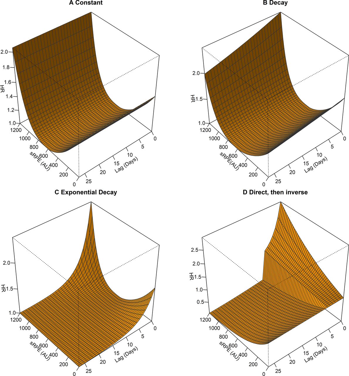
The four simulated relationships between absolute training load and injury risk. The relationships are a combination of the J-shaped function on the absolute training load exposure (figure 2A) and the different functions on the time since training load was sustained (online supplemental figure S3). Training load is measured with the session rating of perceived exertion (sRPE), shown on the x-axis. The time since the current day (day 0) is shown on the y-axis, where 0 is the current day and 27 is the 27th day before the current day. On the z-axis, the risk of injury is measured with the Hazard Ratio (HR), where HR >1 indicates an increased risk, and HR <1 indicates a decreased risk. The four risk shapes are: (A) constant, where the J-shaped risk of training load is constant over time; (B) decay, where the effect size of the J-shaped effect of training load is at its highest on the current day (day 0) and is reduced linearly for each lag day back in time; (C) exponential decay, where the J-shaped risk of training load is at its highest on the current day (day 0) and is reduced exponentially for each lag day back in time; (D) direct, then inverse; where training load linearly increases injury risk during the current week (day 0–6), but linearly decreases injury risk thereafter. This was the shape simulated with a linear model on the absolute training load (online supplemental figure S2B). Training load had no effect after the 27th lag day (4 weeks) in all four scenarios (not shown).
Analyses and simulations were performed using R 4.1.2.20–22 Code and data are available online.23
Step 1: preparing data
Internal training load was measured with the daily session rating of perceived exertion (sRPE)24: the duration of the activity in minutes multiplied by the player’s reported perceived intensity of the activity on a scale from 0 to 10. We simulated a training load study by sampling sRPE values from the observed football dataset. The relative training load from 1 day to the next was calculated with the symmetrized percentage change (%∆sRPE).25 A larger study was simulated: 250 participants (10 football teams), followed for one full season (300 days).
Step 2: simulating time-to-event data
We simulated injuries under different relationship scenarios with the sampled training load. The risk of injury at any given time was predetermined with a time-to-event Cox regression model. Only one injury was simulated per individual. We use the term injury to describe the simulated events. However, the events can also be considered occurrences of pain or other health problems.
The relationship between absolute training load and injury risk was simulated to be J-shaped (online supplemental file 1 figure S2A).15 Under this assumption, the lowest point of risk was intermediate levels of training load. The highest point of risk was set at high levels of training load.

The three simulated relationships between relative training load and injury risk. The relationships are a combination of the linear function on the relative training load exposure (figure 2C) and the different functions on the time since training load was sustained (online supplemental figure S3). Relative training load is measured with the symmetrised percentage change (%Δ) in session rating of perceived exertion (sRPE), shown on the x-axis. The time since the current day (day 0) is shown on the y-axis, where 0 is the current day and 27 is the 27th day before the current day. On the z-axis, the risk of injury is measured with the Hazard Ratio (HR), where HR >1 indicates an increased risk, and HR <1 indicates a decreased risk. The four risk shapes are: (A) constant, where the linear risk of relative training load is constant over time; (B) decay, where the effect size of the linear effect of relative training load is at its highest on the current day (day 0) and is reduced linearly for each lag day back in time; (C) exponential decay, where the linear risk of training load is at its highest on the current day (day 0) and is reduced exponentially for each lag day back in time. Training load had no effect after the 27th lag day (4 weeks) in all three scenarios (not shown).
For relative training load, we simulated a linear relationship with injury risk (online supplemental figure S2C). Higher loads on the current day compared with load on the previous day increased risk, while lower loads on the current day compared with the previous day reduced risk.8
In addition, we simulated the following time-dependent scenarios for both the absolute training load and the relative training load (online supplemental file S3):
Constant. Across 4 weeks (28 days), the effect of training load has a constant effect each day.
Decay. Across 4 weeks (28 days), the effect of training load gradually decays for each day.13 This was hypothesised as a likely scenario if past training load has a direct effect on injury risk.
Exponential decay. On the current day (day 0), training load has the highest risk of injury. The effect of training load drops exponentially the past 4 weeks (28 days). This was hypothesised as a likely scenario if past training load has an indirect effect on injury risk.
Direct, then inverse. Training load values on the current week (acute) increases risk of injury, while the training load values 3 weeks before the current week (chronic) decreases risk of injury (results in supplementary).17 This scenario represents a hypothesis that chronic load is a measure of fitness and absolute acute load is a measure of fatigue.17 High loads relative to the previous time period are thought to increase risk, while low loads relative to the previous time period decrease risk: a linear relationship. Therefore, for this time-lag scenario, we simulated a linear relationship with the absolute training load, and the relative training load was not considered (online supplemental figure S2B).
In summary, seven different relationships between training load and injury risk were simulated (figures 1–2).
Step 3: modelling the time-dependent effect of training load on injury risk
Different methods of modelling training load were compared in their ability to uncover the seven predetermined relationships between training load and injury risk. We chose the most frequently used methods in training load and injury research,26 27 methods proposed as potential alternatives13 16 and a method developed to handle similar challenges in epidemiology.10 Cox regression was used to estimate the relative risk of injury, where internal training load, sRPE or %ΔsRPE was modified or modelled with different methods.
For absolute training load, we modelled the following methods with a quadratic term:
Rolling average (RA).28
Exponentially weighted moving average (EWMA).13
Robust exponential decreasing index (REDI).16
Distributed lag non-linear model (DLNM).10 12
For relative load, we modelled the following methods with a linear term:
Step 4: calculating performance measures to compare methods
We visualised the predicted cumulative risk versus the true cumulative risk in line graphs. The root-mean-squared-error (RMSE), a combined measure of accuracy and precision, was calculated between the predicted and true cumulative hazard. The lower the RMSE, the better the method. We also calculated RMSE on the predicted injury value versus the observed value (the model residuals).
The Akaike’s Information Criterion (AIC) for model fit, coverage of 95% CI, average width of CI and the percentage of simulations where the methods had the lowest RMSE and lowest AIC were also calculated.
Implementation in a handball dataset
The model that performed best in our preliminary analyses of simulated data, the DLNM, was implemented on an actual data set from another team sport, to illustrate how it can be used in practice. To explore the potential for a time-dependent, cumulative effect of training load on health problem risk, we chose a Norwegian elite youth handball cohort (n=205, 36% male, mean age: 17 years (SD: 1), followed 237 days). Although the high amount of missing data (64% of sRPE values) renders it unsuitable for a study of causal inference, it had a sufficient number of health problems for the current methodology study (n=471 health problems).
RPE and duration were collected from the players after each training and match, from which daily sRPE was determined.31 The handball players reported daily whether they had ‘no health problem’ or ‘a new health problem’. Any response of ‘a new health problem’ was considered an event in the current study. Players were encouraged to report all physical complaints, irrespective of their consequences on sports participation or the need to seek medical attention.32
Missing sRPE data were imputed with multiple imputation.33 Cox regression was run with health problem (yes/no) as the outcome and the DLNM of sRPE as the exposure.9 We adjusted for sex and age as potential confounders and included a frailty term to account for recurrent events.34 DLNM combines a function on the magnitude of sRPE and a function of the distance since day 0 up to lag 27 (4 weeks). The sRPE was modelled with restricted cubic splines15 and the lag function with a linear model. The model predictions were visualised to assess the ability of DLNM to explore effects.
Results
Football data simulation
Absolute training load
TheDLNM was the only method that discovered the simulated J-shaped relationship between absolute training load and cumulative risk of injury under all the main time-dependent effects (figure 3). It had, by far, the lowest mean external RMSE (online supplemental file 1 figure S4A-C), the lowest internal RMSE (table 1) and the lowest AIC (online supplemental figure S4D-F). Despite consistently having the narrowest average CI width (≈2 vs >3 (all other methods)), it also had the second-to-highest coverage of 95% CIs under the constant scenario and the highest under the decay scenario (table 1). Except for the exponential decay scenario, all methods had poor coverage overall (<=35%, table 1).

The relationship between absolute training load measured by the session rating of perceived exertion (sRPE) in arbitrary units (AUs) and the risk of injury on the current day (day 0) estimated by four different methods (yellow line), compared with the simulated, true relationship (black line). The y-axis denotes the cumulative hazard – the sum of all instantaneous risks of injury from the past up until the current day. Relationships were simulated under different scenarios, (A–D) constant: the risk of absolute training load is constant over time; (E–H) decay: the effect of absolute training load was at its highest on the current day (day 0) and reduced linearly for each lag day back in time; (I–L) exponential decay: the risk of absolute training load was at its highest on the current day (day 0) and reduced exponentially for each lag day back in time. Methods used to detect these effects were the rolling average, the exponential weighted moving average (EWMA), the robust exponential decreasing index (REDI), and the distributed lag non-linear model (DLNM). Yellow bands are 95% CIs. The figure shows one random simulation of 1900 performed.
Mean performance of methods used to estimate the effect of training load on injury risk (n simulations=1900).
The EWMA was able to detect the exponential decay scenario (figure 3J) and had better accuracy than the rolling average and the robust exponential decreasing index for the decay scenario (figure 3E–G). It had the lowest mean external RMSE and AIC of all three scenarios and methods (table 1, online supplemental figure S4), although, under the constant scenario, the CIs reached negative values (figure 3B).
The rolling average was able to model the constant scenario (figure 3A) and had a mean internal RMSE of 0.113547, slightly lower than EWMA at 0.113548. Under this condition, it had the second best (rank 2) external RMSE in 31% of simulations and third best (rank 3) in 52% of simulations, with similar results for AIC (31% rank 2, 58% rank 3; online supplemental table S1). Here, EWMA was most frequently ranked second best for RMSE and AIC (45% and 39%, respectively (online supplemental table S1).
REDI had consistently the highest mean external RMSE and AIC (online supplemental figure S4, table 1). It was most frequently rank 4 for external RMSE under the constant and decay scenarios and for AIC under all scenarios (online supplemental table S1). Furthermore, REDI consistently had the lowest coverage of 95% CIs (table 1). Instead of discovering that high levels of absolute training load increases injury risk, REDI estimated that high absolute training load decreases injury risk under the exponential decay scenario (figure 3K).
No method was able to accurately model the direct, then inverse scenario (coverage=0%, online supplemental figure S5, online supplemental table S2).
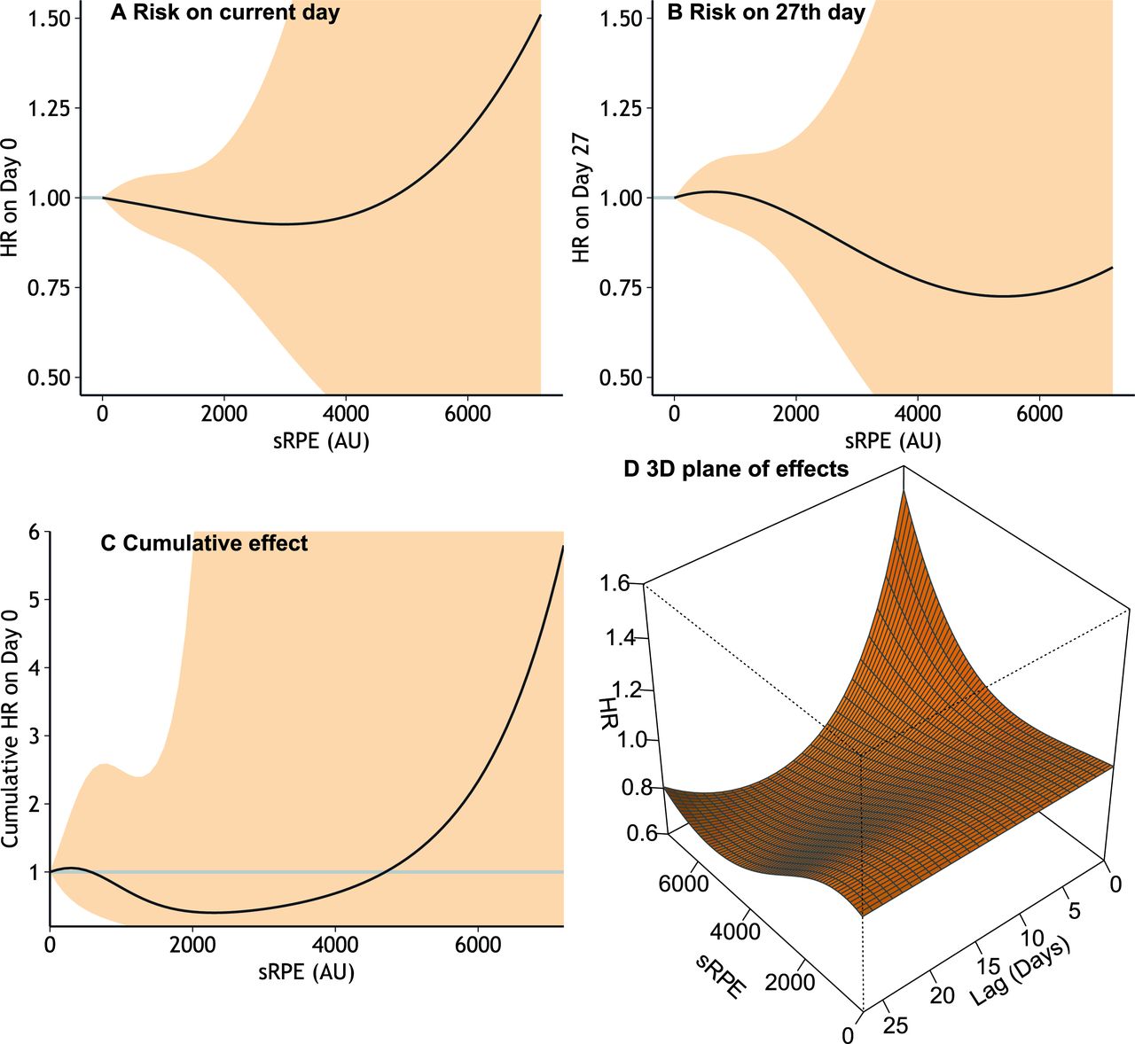
Explorations of the relationship between training load and the risk of suffering a health problem in a Norwegian elite youth handball cohort. Training load is measured by the session rating of perceived exertion (sRPE) in arbitrary units (AUs), shown on all x-axes. The health problem risk is measured by the Hazard Ratio (HR). HR >1 indicates an increased instantaneous health problem risk compared with an individual who had no training load (sRPE=0), <1 a decreased risk. Figure part A shows the risk of a health problem on the y-axis for each level of sRPE on the x-axis, given that the sRPE is sustained on the current day (day 0). Figure part B shows the same figure, given that the sRPE is sustained on the 27th lag day (4 weeks prior). Figure part C shows the cumulative HR – the collective risk of a health problem on the current day given the sRPE sustained in all the days prior to the current day. Finally, figure part D shows the risk relationship between absolute training load (sRPE) on the x-axis and the time since the training was sustained (lag) on the y-axis, where 0 is the current day and 27 is 4 weeks in the past. Risk in HR is on the z-axis. Yellow bands in (A–C) are the 95% CIs surrounding the estimates. The predictions pertain to a 17-year-old female. Based on 471 health problems from 205 handball players.
Relative training load
The Distributed Lag Non-Linear Model (DLNM) was also capable of discovering the cumulative hazard of injury for relative training load (figure 4C, F, I). It had the lowest mean internal RMSE and AIC for the Constant and Decay scenarios (online supplemental figure S6), but for the Exponential Decay scenario, it had the lowest mean AIC and highest internal RMSE (table 1, online supplemental figure S6). Under all scenarios, DLNM had the lowest AIC in nearly 100% of simulations (online supplemental table S3). Although it was most frequently rank 1 internal RMSE for the Constant (52% of simulations) and Decay scenarios (57% of simulations), the rankings varied, and the Acute:Chronic Workload Ratio and Week-to-week %Δ were rank 1 ~23% of the time each (online supplemental table S3).

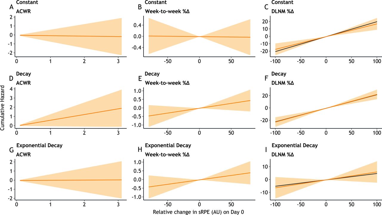
The relationship between relative training load measured in the daily percentage change of session rating of perceived exertion (sRPE) in arbitrary units (AUs) and the risk of injury on the current day (day 0) is estimated by three different methods (yellow line). The y-axis denotes the cumulative hazard – the sum of all instantaneous risks of injury from the past up until the current day. Relationships were simulated under different scenarios, (A–C) constant: the risk of relative training load was constant over time; (D–F) decay: the effect of relative training load was at its highest on the current day (day 0) and reduced linearly for each lag day back in time; (G–I) exponential decay: the risk of relative training load was at its highest on the current day (day 0) and reduced exponentially for each lag day back in time. Methods used to detect these effects were the acute:chronic workload ratio (ACWR), the week-to-week percentage change (%Δ) and the distributed lag non-linear model (DLNM) on daily percentage change Δ%. The DLNM, being on the same scale as the simulation, is also compared with the true, simulated relationship (black line). Yellow bands are 95% CIs. The figure shows one random simulation of 1900 performed.
The Acute:Chronic Workload Ratio (ACWR) and week-to-week %Δ failed to discover a relationship between training load and injury under the Constant scenario (figure 4A, B). ACWR did not find a relationship under the Exponential Decay scenario, either (figure 4G). Both methods had wide confidence intervals, and ACWR fanned to higher uncertainty under higher levels of acute training load relative to chronic training load (figure 4). ACWR had marginally lower internal RMSE and lower AIC than week-to-week %Δ (table 1), and was rank 2 slightly more frequently than rank 3 (online supplemental table S3), except under the Exponential Decay scenario where the opposite was the case.
Handball example data analysis
The Distributed Lag Non-linear Model indicated, with high uncertainty, an increased risk of a health problem on the current day (HR (HR)>=1.2) for players with high internal load (sRPE above 4 000, figure 5A). This tapered to no effect if the training load was performed around a week ago (6 days before the current day, figure 5D), to a decreased risk of health problems the further in the past high training loads were sustained, to a HR of 0.75 on the 27th day before the current day (figure 5B). The cumulative risk was increased if an individual performed no training in the past and had high internal training load on the current day (figure 5C). None of the effects were significant (p>=0.8) and confidence intervals were broad (online supplemental table S4).
Discussion
This is the first simulation study to explore methods for assessing the cumulative effect of long-term training load on injury or health problem risk in team sports. The Distributed Lag Non-linear Model (DLNM) had the highest combined accuracy and precision, the highest certainty, and the best model fit for almost all studied scenarios. It was the only method capable of exploring both the effects of the magnitude of training load and the time-dependent effects of past training load exposure.
In the application of DLNM on a handball cohort, we were hampered by poor data quality. Also, due to anonymization, few covariates were available for confounder adjustment. The effects may have been spurious. We have included the analysis only as an illustration of how to use the DLNM in practice.
Modelling methods for absolute training load
For determining the cumulative effect of the absolute training load, the Rolling Average was outclassed by the Exponentially Weighted Moving Average (EWMA). When the effect of absolute training load was simulated to be the same regardless of the distance in time since the current day – the scenario in which Rolling Average was thought to be appropriate – Rolling Average was only marginally better than the EWMA. EWMA had a better fit under the more realistic scenarios where the effects of training load decayed based on distance in time, both linearly and exponentially. This is in line with the concerns raised by Menaspà,28 that the rolling average fails to take into account that training load performed in the past contributes less to injury risk than recent training load
The Robust Exponential Decreasing Index (REDI) was also outperformed by EWMA, under both scenarios where the training load effect decayed based on distance in time. Across the board, REDI had the highest RMSE, highest AIC, and lowest coverage of 95% confidence intervals. Although it had better RMSE under the Exponential Decay scenario than the rolling average, it erroneously estimated that higher internal training loads decreased injury risk (inverse relationship), when it was actually the opposite (ie, higher training load increased injury risk). REDI has previously been compared on observed training load values where the true relationship between training load and injury was unknown,35 and it was recommended for its ability to handle missing data.16 We believe that using imputation methods is more suitable for longitudinal data,33 and in such cases, the advantage of specifying weights on missing observations is no longer applicable. REDI was among the methods that do not require a full time period (ie, 28 days) before the first calculation, but for comparability, we had to run it with the same limitation as the other methods. Arguably, it may therefore have performed better in a real study. On the other hand, this would also have been the case for the Distributed Lag Non-Linear Model (DLNM), which was vastly superior to all other methods analysed, even with this constraint.
DLNM had the lowest mean RMSE, AIC, and narrowest 95% CI width compared with the other three methods for all scenarios. The DLNM was the only method that did not require subjective aggregation. Aggregation distillates the information available in the data to a summary, and these summaries are all the Cox regression model must work with. This increases the uncertainty of the estimates. In contrast, DLNM uses all the information available in the data.12 Furthermore, no subjective determination of time-lag weights is required. Using splines or fractional polynomials, it can explore non-linearity in both the magnitude of the effect of absolute training load and in the time-dependent effects.15
While it performed best compared with other methods, DLNM was unable to model the “Direct, then inverse” scenario. This scenario was built on the theory that training load exposure the current week increase risk while those sustained the previous 3 weeks reduce risk.8 Higher sample sizes than those in the current simulation may be needed to discover such a complex shape, if it were to exist. The splines may have required more than three knots, and linear splines may have been a better option than cubic splines to discover the sudden change in direction of effect.
Modelling methods for relative training load
Studying the relative training load proved challenging, as all methods compared were on different scales. According to the AIC, the most comparable metric,12 DLNM had the best model fit under all scenarios. Given that we simulated an effect on the risk of injury based on the symmetrized percentage change from 1 day to the next, this was to be expected. The week-to-week percentage change and ACWR assume that day-to-day differences are of little to no importance. Currently, the time-period of relative training load that is relevant towards injury risk is debatable36; a calendar week may be arbitrary for many sports. We argue that if DLNM can detect the effect of day-to-day relative change, it should be flexible enough to detect less granular effects. In particular, team sports such as football often operate in micro-cycles of days since the previous match up to and including the next match.15 However, it would still be up to the researcher to calculate percentage changes on time periods of their choosing before running DLNM, with the inherent difficulties of ratios.25
Even with the symmetrized percentage change, the percentage change cannot be calculated if the numerator or denominator is zero. Recovery days are an important aspect of training load history and must be evaluated to fully understand the effects of training load. This is a challenge that remains unsolved.
An application of distributed lag non-linear models in handball
The Distributed Lag Non-linear Model was able to explore non-linear time-dependent effects in the observed Norwegian youth elite handball data. The results had a high degree of uncertainty (p>=0.8), and we caution against considering them as evidence of a causal or associative relationship. They nevertheless illustrate how DLNM can be used in practice. DLNM can show how different levels of training load affects risk, and also how the effects changes with the distance in time since the training load exposure. It can also show the combined effect of these two dimensions and estimate the cumulative effect. However, performing DLNM and the corresponding visualisations in a training load and injury or health problem risk study may require collaboration with a statistician.37 In addition, large sample sizes and good data quality may be needed to meet the complexity of the training load and injury risk relationship. In the handball data, 471 health problems occurred in 205 participants. As this was insufficient, future research may require even more participants for an accurate measure of effect.
Limitations
To feasibly analyse all results in a single article, we had to limit the number of methods compared in the simulations. This meant that two recently-proposed methods of relative training load were not among the compared methods.38 39 Additionally, different variants of the ACWR were not considered, as these have been explored extensively in other studies.30 40
All methods in the simulation were run with the same specification for all scenarios to ensure consistency and comparability. In a real study, clinical rationale and hypothesis, as well as sensitivity analyses of model fit, would aid in determining the number and location of knots in splines for DLNM, the lambda value for EWMA and REDI, and the time-periods for RA, EWMA, REDI and ACWR. Therefore, the flexibility of methods was not fully explored. In addition, for the relative training load, the simulation assumed that daily differences had an effect, an assumption that favoured DLNM, which has superior flexibility compared with the other methods. This advantage may be less prominent if stricter assumptions (ie, differences at the micro-cycle level) can be made15; however, we believe that the flexibility of the DLNM is one of its greatest strengths, rendering it useful in a wide range of situations.
Conclusion
The Distributed Lag Non-Linear Model is ideal for exploring the cumulative effect of the absolute training load and relative training load on injury risk, while accounting for time-dependent effects. For causal studies where training load is not the exposure of interest, but a confounder in need of adjustment, using the Exponentially Weighted Moving Average for the absolute training load is an alternative.
Data availability statement
Data are available in a public, open access repository. Data are available upon reasonable request. All data relevant to the study are included in the article or uploaded as supplementary information. All data relevant to the study are included in the article, are available as supplementary files, or available upon reasonable request. The anonymous training load variable from the Norwegian Premier League football data, and all statistical programming code, is available in a GitHub repository. The anonymised Norwegian elite youth handball data are available upon reasonable request.
Ethics statements
Patient consent for publication
Ethics approval
This study involves human participants and was approved by The Norwegian Premier League football study and Norwegian elite youth handball study was approved by the Ethical Review Board of the Norwegian School of Sport Sciences, and by the Norwegian Centre for Research Data, with registration numbers 722773, and 407930, respectively. Participants gave informed consent to participate in the study before taking part.
Acknowledgments
We thank Christian Thue Bjørndal for granting access to the Norwegian elite youth handball data. We also thank Garth Theron for programming the Norwegian Premier League database. This research would not be made possible without the collaboration of coaches and athletes, and we thank the participants who contributed.
References
Supplementary materials
Supplementary Data
This web only file has been produced by the BMJ Publishing Group from an electronic file supplied by the author(s) and has not been edited for content.
Footnotes
Twitter @lena_kbm, @torsteindalen
Contributors All authors conceptualized the study. Authors TEA, TD-L, and BC determined the aim and scope of the study, and the study design, with input from LKB-M and MWF. Author LKB-M performed simulations, statistical analyses, and wrote the manuscript under supervision from authors MWF and TEA. All authors contributed with notable critical appraisal of the text and approved the final version. LKB-M was the guarantor of this study.
Funding The Oslo Sports Trauma Research Centre provided all funding for performing this study. The Oslo Sports Trauma Research Center has been established at the Norwegian School of Sport Sciences through generous grants from the Royal Norwegian Ministry of Culture, the South-Eastern Norway Regional Health Authority, the International Olympic Committee, the Norwegian Olympic Committee & Confederation of Sport, and Norsk Tipping AS.
Competing interests None declared.
Patient and public involvement Patients and/or the public were not involved in the design, or conduct, or reporting, or dissemination plans of this research.
Provenance and peer review Not commissioned; externally peer reviewed.
Supplemental material This content has been supplied by the author(s). It has not been vetted by BMJ Publishing Group Limited (BMJ) and may not have been peer-reviewed. Any opinions or recommendations discussed are solely those of the author(s) and are not endorsed by BMJ. BMJ disclaims all liability and responsibility arising from any reliance placed on the content. Where the content includes any translated material, BMJ does not warrant the accuracy and reliability of the translations (including but not limited to local regulations, clinical guidelines, terminology, drug names and drug dosages), and is not responsible for any error and/or omissions arising from translation and adaptation or otherwise.